DYNAMICAL SYSTEMS Tutorial 11

Functions and Variables Used in This Tutorial

arrowflag, arrowvec, classify2D, labshift, liaparmval, liaparmvec, liapcontours, liapsign, liapsignseq, orbdt,
orbdtval, parmval, parmvec, plotreset, plrange, portrait, setparm, setstate, slopevec, statevec, sysid, and sysname.

Description of Systems Used in This Tutorial

In this tutorial, we use Liapunov functions to look at the stability of some planar equilibria. The routines
demonstrated here do not help in the selection of a trial form for a Liapunov function, but they do allow a quick graphical
check on the sign of either the function or its orbital derivative. As examples, we use two simple nonlinear systems for
which linearization does not yield a definite answer on the stability question. Both systems are centers in linear theory.

First Example

We define a simple nonlinear system with one equilibrium, at x = y = 0.

setstate[{x,y}];

setparm[{a}];

slopevec = {-2*y-x^3, a*x - y^3};

parmval = {1};

sysname = "Liap1";

We first try classify2D.

classify2D[{0,0}]

Abbreviations used in classify2D.

L = linear, NL = nonlinear, R2 = repeated root.

Z1 = one zero root, Z2 = two zero roots.

This message printed once.

stable (L), indeterminate (NL) - center

Thus the linearized system is a stable center, so there is no conclusion about the stability of the nonlinear system. We now
try to find a Liapunov function V. We can establish stability of the equilibrium if we find a V which (1) is positive definite
in a deleted neighborhood of the origin and which (2) has a negative definite orbital derivative in a deleted neighborhood of
the origin. Liapunov functions are defined as expressions in the state variables and any parameters that we wish to include.
We try a simple quadratic function with one parameter.

Vliap = x*x + α*y*y;

This is clearly positive definite for any positive alpha. We next declare the parameter alpha as a Liapunov parameter, and
set the parameter value to 1.

liaparmvec = {α};

liaparmval = {1};

Now we look at the orbital derivative of this function.

orbdt[Vliap]

2 x (-x³ - 2 y) + 2 y (a x - y³) α

To get the orbital derivative with the current system parameters substituted, we use orbdtval.

orbdtval[Vliap]

2 x (-x³ - 2 y) + 2 y (x - y³)

We see that a and alpha have been replaced by their present values (1 in both cases).

To get a quick look at the sign of the orbital derivative, we use the function liapsign, which will give us a contour
with regions of positive function in white, negative in grey. This routine automatically substitutes current values of both
system and Liapunov parameters.

plrange = {{-1.5,1.5},{-1.5,1.5}};

liapsign[orbdt[Vliap]]

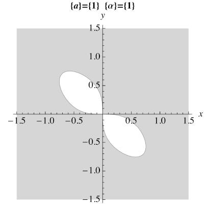
We see that this is not a suitable Liapunov function because the orbital derivative takes on both signs. We now use
the function liapsignseq to construct a sequence of such graphs, for a sequence of values of the parameter in the Liapunov
function. We try the values α = 1, 2, and 3.

parmlist = {1,2,3};

liapsignseq[parmlist,orbdt[Vliap]]

Liapunov Sequence for 2 x(-x³ - 2 y) + 2 y (a x - y³) α

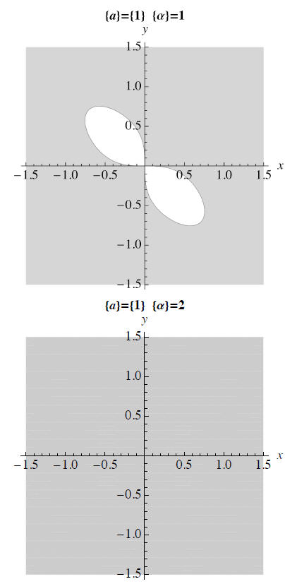
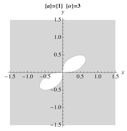
Within the limits of the graphical resolution, it looks like α = 2 may work. Let's see if we can verify this
analytically.

liaparmval = {2};

orbdtval[Vliap]

2 x (-x³ - 2 y) + 4 y (x - y³)

Simplify[%]

-2 (x⁴ + 2 y⁴)

Now we have shown analytically that α = 2 gives us a valid Liapunov function, and the equilibrium at {0,0} is
therefore strictly stable. In fact the analytical formulas show that the equilibrium is a global attractor for the system.

We can look at the contours of both the Liapunov function and its orbital derivative by using the plotting function
liapcontours.

liapcontours[Vliap]


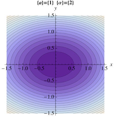
liapcontours[orbdt[Vliap]]


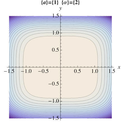
Before leaving this example, lets see what the solution looks like near the equilibrium. We look at a phase portrait
with four different initial conditions.

intlist = {{1,1},{-1,1},{-1,-1},{1,-1}};

h = 0.05;

nsteps = 300;

t0 = 0.0;

arrowflag = True;

arrowvec =

portrait[intlist,t0,h,nsteps,1,2]


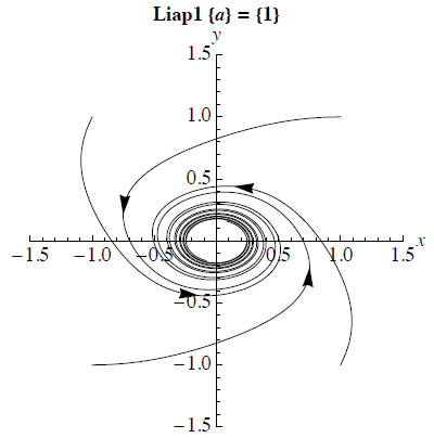
Now we see that the equilibrium is a nonlinear spiral. If we continued the integration the orbits would eventually
approach the origin, but the process is very slow because the approach is driven by terms which are cubic in the distance
from the origin.

Second Example

In this example, we consider a simple nonlinear system without any parameters.

setstate[{x,y}];

setparm[{}];

parmval = {};

slopevec = {y-x*(x^2+y^2)-5*(x*y)^2,-x-y*(x^2+y^2)};

sysname = "Linear Center";

We start by looking at equilibrium by linearization.

classify2D[{0,0}]

stable (L), indeterminate (NL) - center

As before we get a linear center, which is indeterminate for our nonlinear system. We try a simple Liapunov function.

Vliap2 = x^2+y^2;

liaparmvec = {};

liaparmval = {};

Now we look at the sign of the orbital derivative.

orbdt[Vliap2]

2 x (y - 5 x² y² - x (x² + y²)) + 2 y (-x - y (x² + y²))

Simplify[%]

-2 (x⁴ + 2 x² y² + 5 x³ y² + y⁴)

plrange = {{-2,2},{-2,2}};

liapsign[orbdt[Vliap2]]

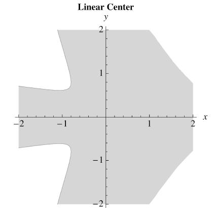
We see that the orbital derivative is not negative everywhere. However, it is negative definite in a neighborhood of
the origin, so this establishes the local strict stability of the equilibrium there. This calculation leaves open the question of
whether the origin is a global attractor for the system. Lets look for other equilibria.

othereq = nfindpolyeq

{{881.08383 - 1.51709 i, -0.298048 - 0.488556i },
{81.08383 + 1.51709 i, -0.298048 + 0.488556 i}, {-1.28523, 0.628076},
{8-0.818705, 0.703033i, 80.0242891 - 0.455594 i}, {-0.747539 + 0.321368 },
{80.0242891 + 0.455594 i, -0.747539 - 0.321368 i},
{80.372109 - 0.207366 i, 0.506403 + 0.654794i },
{80.372109 + 0.207366i, 0.506403 - 0.654794i },
{8-0.428263 + 0.325725 i, -0.12637 + 0.770525i },
{8-0.428263 - 0.325725 i, -0.12637 - 0.770525i }, {0., 0.}

We see that there are two other real equilibrium points. We check their stability.

classify2D[{-1.28523, 0.628076}]

strictly stable - spiral

classify2D[{-0.818705, 0.703033}]

unstable - saddle

Thus the equilibrium at {-1.28523, 0.628076} is also an attractor.

Exercise

This problem is taken from Chapter 10 of Nonlinear Ordinary Differential Equations, (second edition), D.W.
Jordan and P. Smith, Oxford Press, 1987. Consider the system defined by statevec = {x,y}, slopevec = {-x³ + y⁴, -y³ + y⁴}.
Show that linearization leads to no conclusion for the stability of the origin. Find a Liapunov function which proves
stability. Use liapsign to check the sign of the orbital derivative.